Recently, I’ve been exploring some different gridded daily precipitation datasets and evaluating how they impact watershed models I’ve been working on. Let’s explore using the rayshader to make some three-dimensional maps.
First, obtain the gridded precipitation data. I will use the 30-yr mean annual precipitation from PRISM. Luckily, there is an R package so we can easily script the data download.
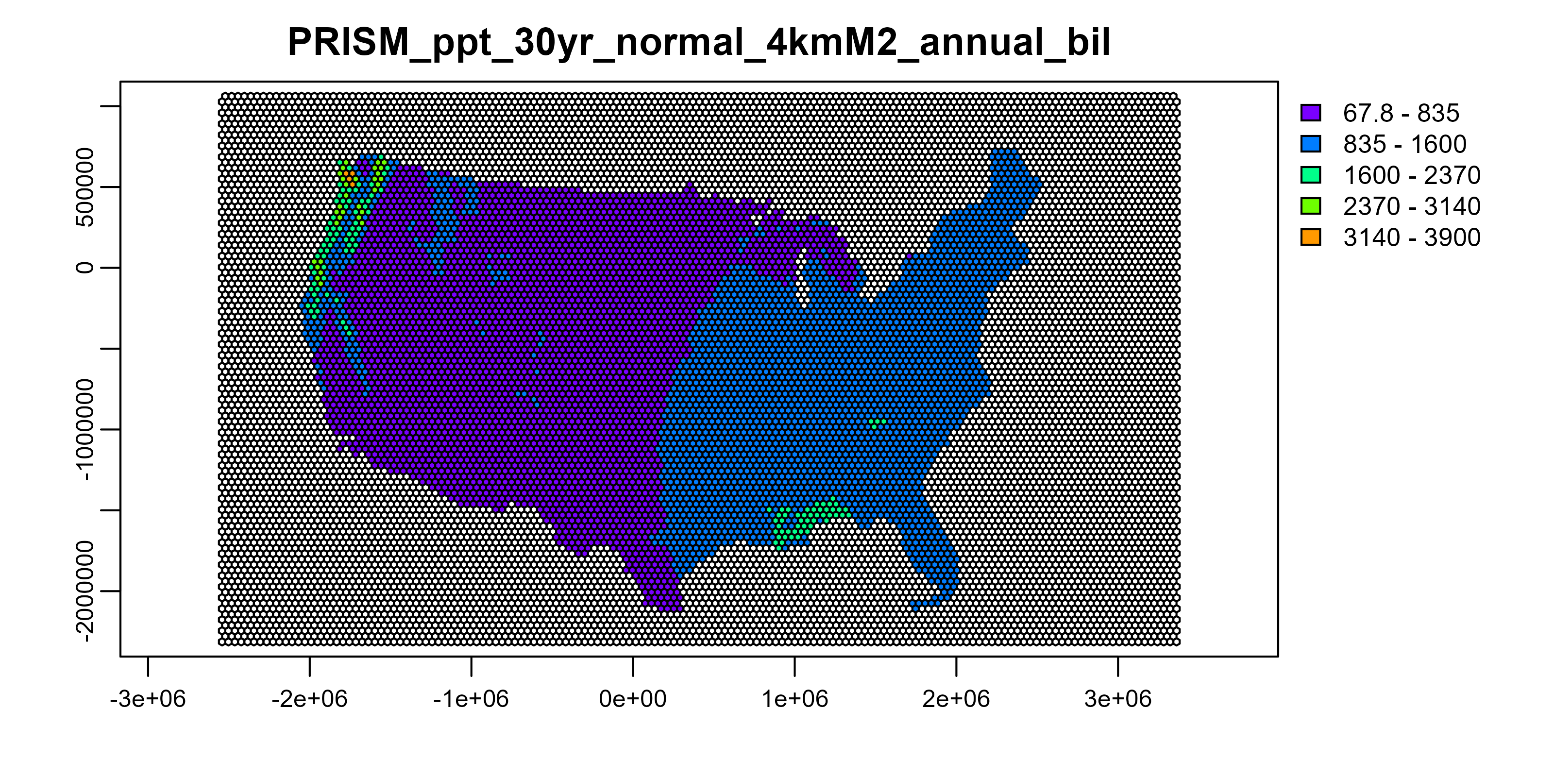
Second, I will smooth the data a little bit by summarizing into tiles. There is a lot of variation at the nation-wide scale by spatially-binning and averaging the data, the map is just a little more aesthetically pleasing to my eye. This can be done a bunch of different ways. Here, I will use the sf and terra packages to create and populate the hexagons with mean annual precipitation data.
Third, I will render a three-dimensional map with rayshader. So, load the necessary packages before we start. I’m using the development version of rayshader and rayrender because of some massive speed improvements, I recommend installing if you can (remotes::install_github(tylermorganwall/rayshader); remotes::install_github(tylermorganwall/rayrender)). statesRcontiguous is only on Github, so install as follows: remotes::install_github(charliejhadley/statesRcontiguous).
Download Data
The prism package downloads the gridded precipitation datasets we request, then stores the path so we can read with the rast function. I’m downloading the 4km resolution data, if you were doing this at the state or local level, consider downloading the 800m dataset for better resolution.
## PRISM data
tmpdir <- tempdir()
prism_set_dl_dir(tmpdir)
prism <- get_prism_normals("ppt", "4km", annual = TRUE, keepZip = FALSE)
  |
  |                                                            |   0%
  |
  |============================================================| 100%
prism_rast <- prism_archive_subset("ppt", "annual normals", resolution = "4km")
prism_rast <- pd_to_file(prism_rast)
prism_rast <- rast(prism_rast)
prism_rast <- project(prism_rast, "+proj=laea +lat_0=45 +lon_0=-100 +x_0=0 +y_0=0 +a=6370997 +b=6370997 +units=m +no_defs ")
Tile rasters
As I mentioned, there are various ways to make the tiles.[@cstats1](https://twitter.com/cstats1) posted an efficient workflow using the summary_stat function in ggplot. I wanted to project the data and utilize the new terra package to summarize the data. It take a bit longer, but I like the results.
Since several people have asked and I have no idea when I will actually get around to writing this process up, here are the steps to making elevation tiles in #rayshader sans pulling in the shapefiles and elevation data directly from #rstats using the Monterey Bay elevation file pic.twitter.com/0aeXnCEIk0
— newishtodc (@cstats1) February 22, 2021
## create and extent polygon
prism_ext <- as.polygons(ext(prism_rast), crs=crs(prism_rast))
prism_ext <- st_as_sf(prism_ext)

## create a hexagon grid in the extent polygon
hexagons <- st_make_grid(prism_ext,
                         n = c(150,150),
                         square = FALSE,
                         crs = crs(prism_ext))

## convert from sf back to terra,
## we lose the crs def along the way
## so set the crs again
hexagons <- vect(hexagons)
crs(hexagons) <- crs(prism_rast)

## calculate the mean raster values in each polygon
prism_summary <- extract(x = prism_rast,
                         y = hexagons,
                         fun = mean,
                         na.rm = TRUE)

## extract returns a matrix, need to get the data back
## into hexagons
values(hexagons) <- data.frame(ID = 1:nrow(hexagons))
hexagons <- merge(hexagons, data.frame(prism_summary))
values(hexagons) <- data.frame(prism_summary)

## what does it look like?
plot(hexagons, "PRISM_ppt_30yr_normal_4kmM2_annual_bil")

Rayshade
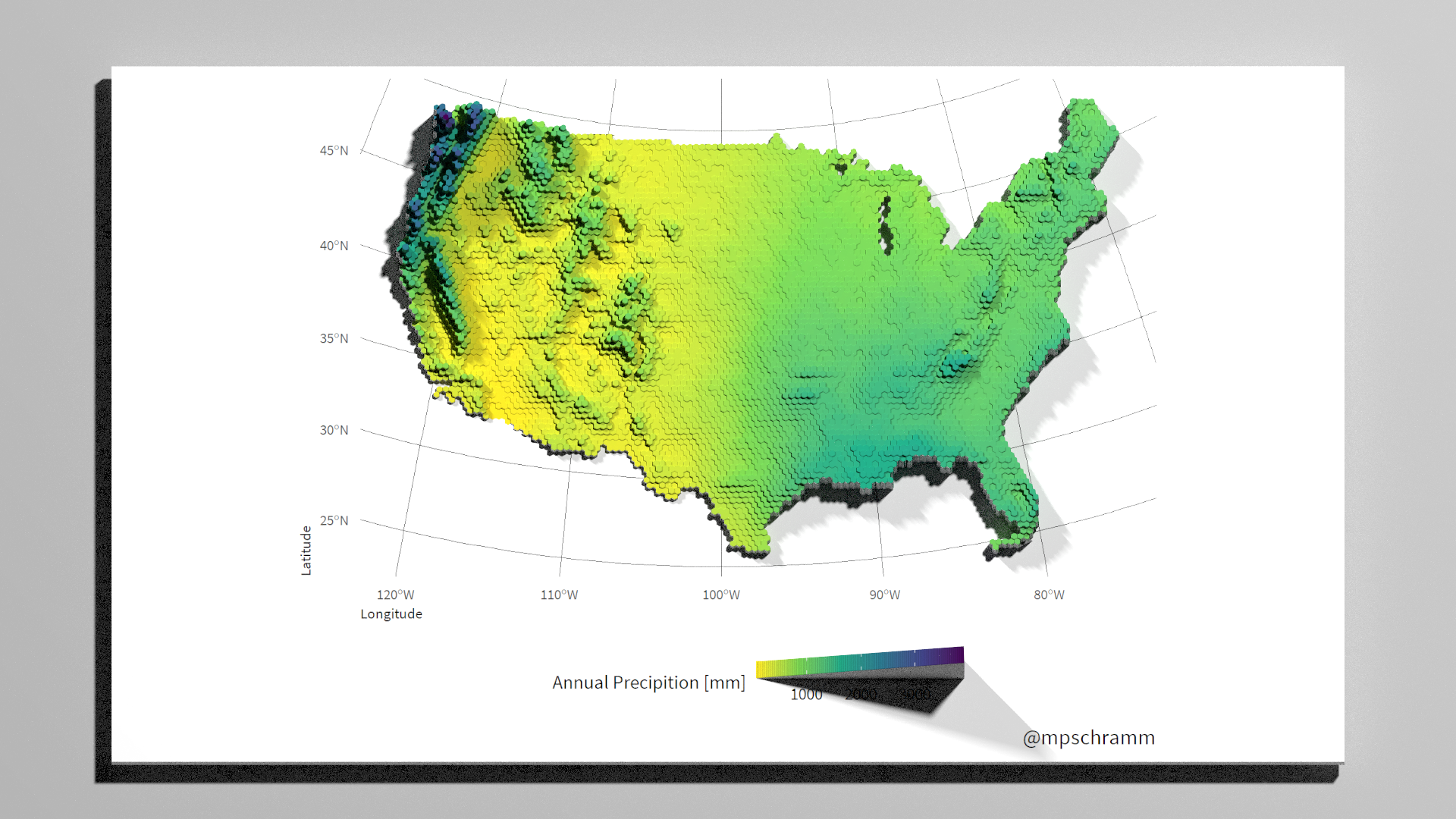
Time to make the computer go bananas. First, convert hexagons to sf and plot with ggplot2. Then we can easily generate a rayshaded plot. If you want to forgo, ggplot2, convert to a raster and run through rayshader. I usually render a low res version first to make sure I like the colors, scaling, etc. These can take quite some time to render. Play with the settings to get what you like and share on Twitter with #rayshader.
ggplot2
## convert to sf and features with NA values
hexagons <- st_as_sf(hexagons) %>%
  filter(!is.na(PRISM_ppt_30yr_normal_4kmM2_annual_bil))

## make your ggplot, customize as needed
ggplot(hexagons) +
  geom_sf(aes(fill = PRISM_ppt_30yr_normal_4kmM2_annual_bil), color = NA) +
  scale_fill_viridis_c("Annual Precipition [mm]", direction = -1) +
  labs(x = "Longitude", y = "Latitude", caption = "@mpschramm") +
  theme(text = element_text(family = "Source Sans Pro"),
        legend.position = "bottom",
        legend.title = element_text(size = 8),
        legend.text = element_text(size = 7),
        legend.key.height = unit(0.25, "cm"),
        panel.background = element_rect(fill = "white", color = "white"),
        panel.grid = element_line(color = "grey10",
                                  size = .1),
        axis.title.x = element_text(size = 6, hjust = 0),
        axis.title.y = element_text(size = 6, hjust = 0),
        axis.text.x = element_text(size = 6),
        axis.text.y = element_text(size = 6),
        axis.ticks.x = element_blank(),
        axis.ticks.y = element_blank()) -> p1

## make 3D ggplot
plot_gg(p1,
        multicore = TRUE,
        width = 4*1.777,
        height = 4,
        solidcolor = "white",
        theta = 0,
        phi = 80,
        fov = 0,
        zoom = .5,
        background = "grey80",
        windowsize = c(1920,1080))

## brrrrrr
render_highquality(lightdirection = 45,
                   lightaltitude = 60,
                   lightintensity = 1000,
                   samples = 1000, #lower this to get faster rendering
                   sample_method = "sobol",
                   parallel = TRUE,
                   width = 1920,
                   height = 1080,
                   ground_material = rayrender::diffuse(color = "grey40"),
                   clear = TRUE)

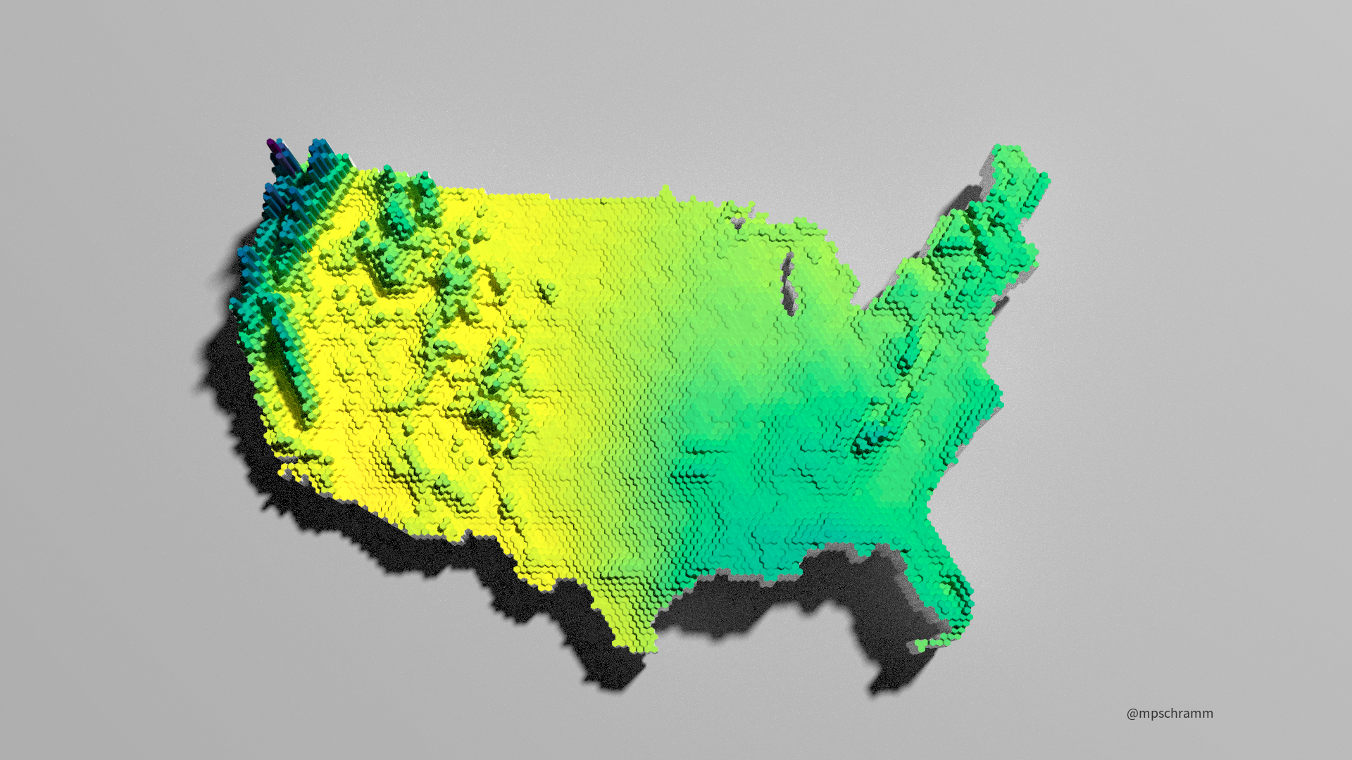
base/sp
## rasterize hexagons:
hexagons <- vect(hexagons)
crs(hexagons) <- crs(prism_rast)
hexagons <- rasterize(hexagons, prism_rast,
                      field = "PRISM_ppt_30yr_normal_4kmM2_annual_bil")
# convert from SpatRast to Raster to matrix
pptmat = raster_to_matrix(raster::raster(hexagons))
pptmat %>%
  height_shade(texture = hcl.colors(100, palette = "viridis", rev = TRUE)) %>%
  plot_3d(pptmat,
          zscale = 16,
          solidcolor = "white",
          theta = 0,
          phi = 80,
          fov = 45,
          zoom = .5,
          background = "grey80",
          windowsize = c(1920,1080))
render_highquality(lightdirection = 45,
                   lightaltitude = 60,
                   lightintensity = 900,
                   samples = 3000,
                   sample_method = "sobol",
                   parallel = TRUE,
                   width = 1920,
                   height = 1080,
                   ground_material = rayrender::diffuse(color = "grey40"),
                   clear = TRUE)
