Combine a hydrograph and hyetograph in ggplot2

Streamflow hydrographs and precipitation hyetographs are commonly combined into one plot by hydrologists. Here is one way to make these plots in R.

It isn’t entirely uncommon to come across a streamflow hydrograph combined with a precipitation hyetograph. Although the general wisdom is to avoid combining data of different scales on one graph, this practice seems accepted in the hydrology commuinity, in particular with the precipitation represented along the top of the plot. I’m not one to judge.

Here is an approach to do it with ggplot and cowplot.

This example uses “instantaneous” discharge and precipitation data obtained from the USGS via the amazing dataRetrieval package.

library(dataRetrieval)
library(tidyverse)
library(lubridate)
library(cowplot)

## download some example data
site <- "08105872"

discharge <- readNWISuv(siteNumbers = site,
                        parameterCd = "00060",
                        startDate = "2022-03-17",
                        endDate = "2022-07-15")
discharge <- renameNWISColumns(discharge)

precip <- readNWISuv(siteNumbers = site,
                        parameterCd = "00045",
                        startDate = "2022-03-17",
                        endDate = "2022-07-15")
precip <-renameNWISColumns(precip)

## join the discharge and precip by date

joined_data <- discharge |> 
  left_join(precip |>  select(dateTime, Precip_Inst), 
            by = c("dateTime" = "dateTime"))

Streamflow is plotted normally using ggplot(). I’m am taking the time to move labels and legends where I want them in the final figure, so bear with me.

p1 <- ggplot(joined_data) +
  geom_line(aes(dateTime, Flow_Inst, color = "Discharge")) +
  scale_y_continuous(position = "left",
                     limits = c(0, 1000),
                     expand = c(0,0)) +
  scale_color_manual(values = c("steelblue")) +
  guides(x = guide_axis(angle = 90)) +
  labs(y = "Discharge [cfs]",
       x = "Date") +
  theme_minimal() +
  theme(axis.title.y.left = element_text(hjust = 0),
        legend.position = "bottom",
        legend.justification = c(0.25, 0.5),
        legend.title = element_blank())
p1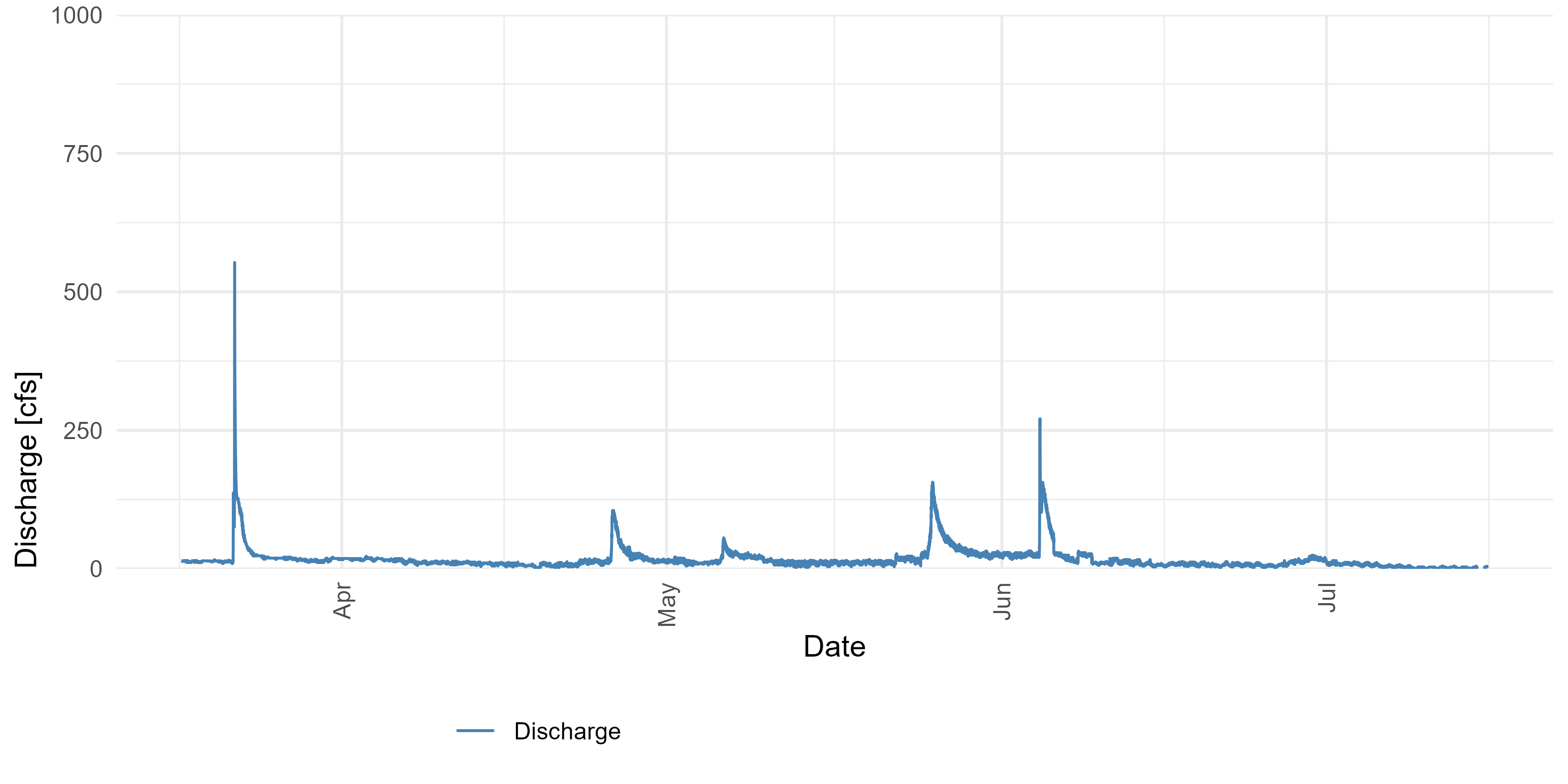

Precipitation will be plotted from the top down. Here, I’m using a line graph since it is the easiest way to start.

p2 <- ggplot(joined_data) +
  geom_line(aes(dateTime, Precip_Inst, color = "Precip")) +
  scale_y_reverse(position = "right",
                  limits = c(10,0),
                  breaks = c(0,0.25,0.5),
                  labels = c(0,0.25,0.5),
                  expand = c(0,0)) +
  scale_color_manual(values = c("sienna1")) +
  guides(x = guide_axis(angle = 90)) +
  labs(y = "Precipitation [inches]", x = "") +
  theme_minimal() +
  theme(axis.title.y.right = element_text(hjust = 0),
        legend.position = "bottom",
        legend.justification = c(0.75, 0.5),
        legend.title = element_blank())
p2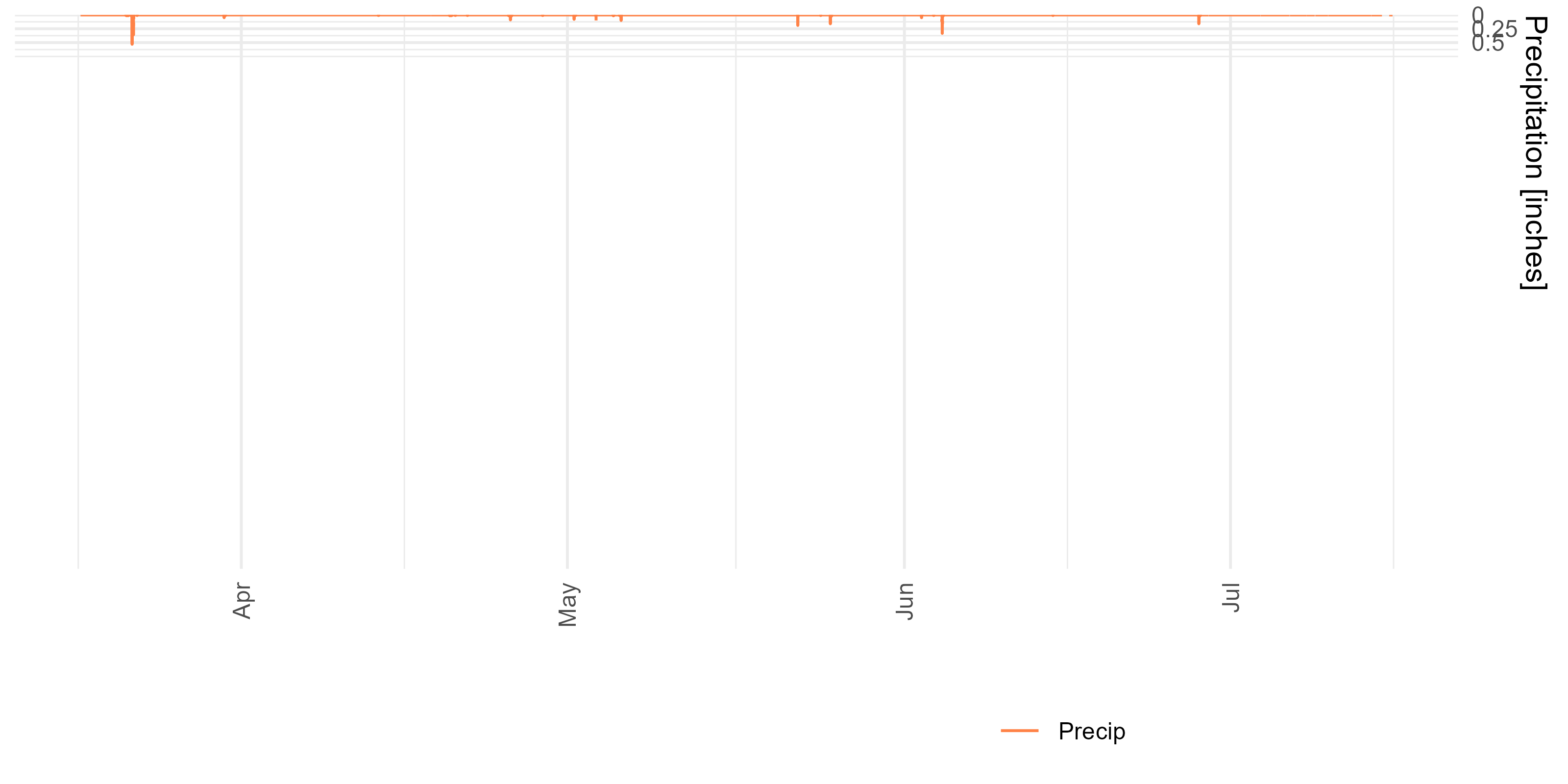

Now we can use cowplot and the align_plots() function to combine things.

aligned_plots <- align_plots(p1, p2, align = "hv", axis = "tblr")
out <- ggdraw(aligned_plots[[1]]) + draw_plot(aligned_plots[[2]])
out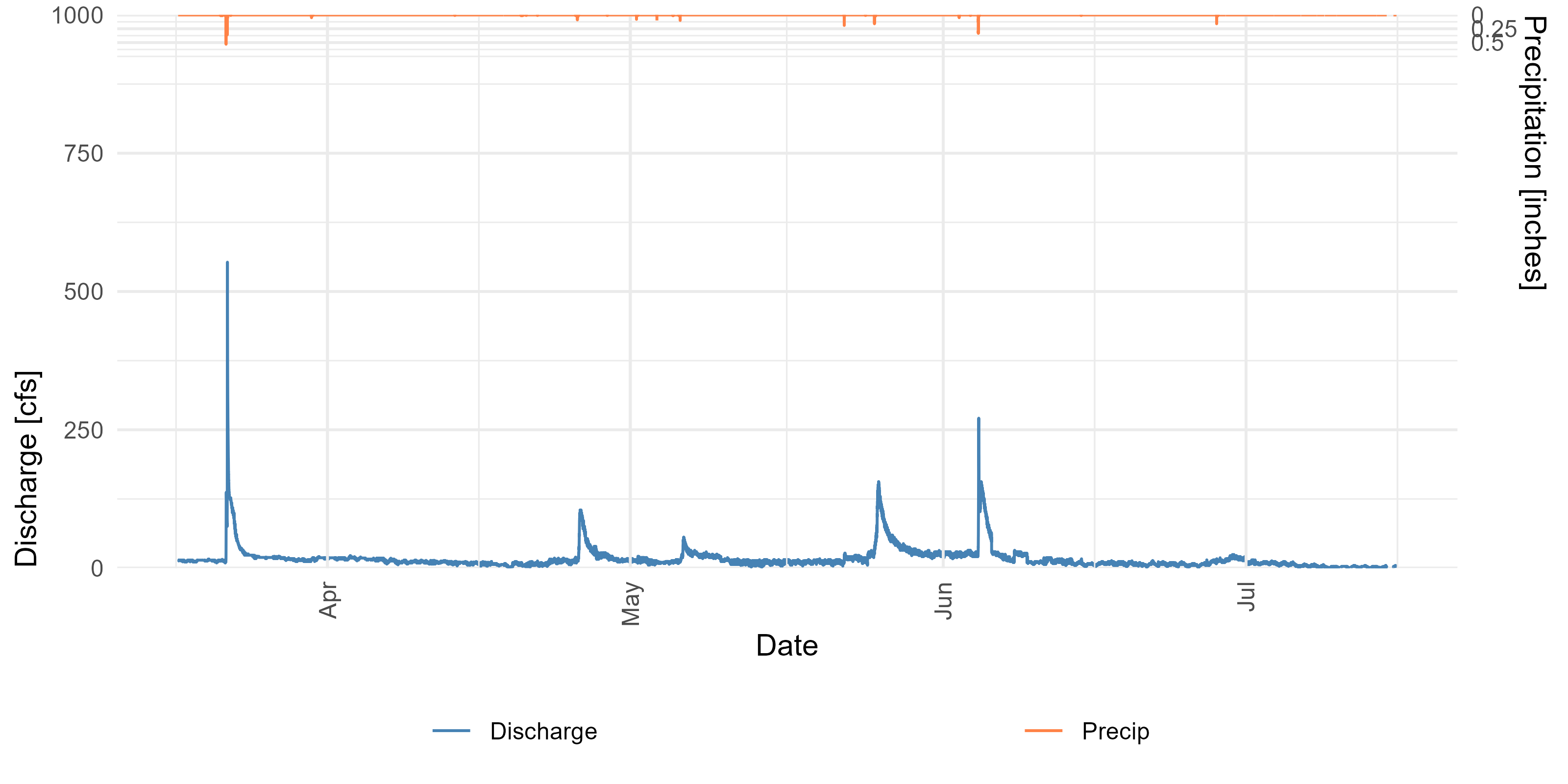

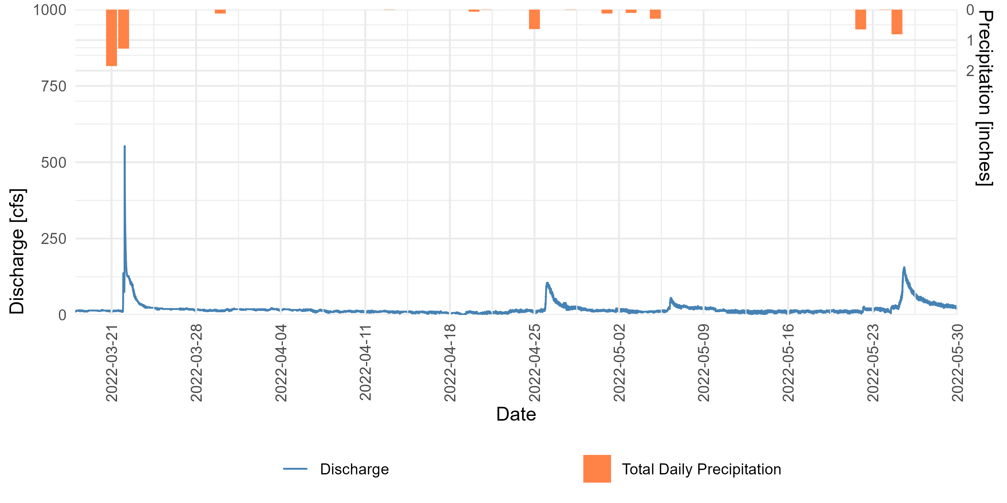
This doesn’t technically include a hyetograph, which is a histogram of streamflows. It take a little more care to ensure the x-axis on both graphs line up if you want to aggregate precipitation. For simplicity, this example aggregates streamflow by day. Essentially, use the scale_x_date() and scale_x_datetime() functions to set common limits and breaks. This should adapt to most situations.

p1 <- p1 + 
  scale_x_datetime(date_breaks = "week",
               limits = c(as.POSIXct("2022-03-18", tz="UT"), 
                          as.POSIXct("2022-05-30", tz="UT")),
               expand = c(0,0)) 

total_precip <- precip |> 
  mutate(date = as.Date(dateTime)) |> 
  group_by(date) |> 
  summarise(Precip = sum(Precip_Inst))

p3 <- ggplot(total_precip) +
  geom_col(aes(date, Precip, fill = "Total Daily Precipitation")) +
  scale_y_reverse(position = "right",
                  limits = c(10,0),
                  breaks = c(0,1,2),
                  labels = c(0,1,2),
                  expand = c(0,0)) +
  scale_x_date(date_breaks = "week",
                   limits = c(as.Date("2022-03-18"), 
                              as.Date("2022-05-30")),
               expand = c(0,0)) +
  scale_fill_manual(values = c("sienna1")) +
  guides(x = guide_axis(angle = 90)) +
  labs(y = "Precipitation [inches]", x = "") +
  theme_minimal() +
  theme(axis.title.y.right = element_text(hjust = 0),
        legend.position = "bottom",
        legend.justification = c(0.75, 0.5),
        legend.title = element_blank())

aligned_plots <- align_plots(p1, p3, align = "hv", axis = "tblr")
ggdraw(aligned_plots[[1]]) + draw_plot(aligned_plots[[2]])