Time-series decomposition and trend analysis in Python

Decompose time series in Python and a function for the Mann-Kendall test for trend.

There are a number of methods to accomplish time-series decompositions in R, including the decompose and STL commands.

I haven’t come across a seasonal decomposition method in Python comparable to R’s STL. However, statsmodels 0.6 added a naive seasonal decomposition method similar to R’s decompose that is not as powerful as the LOESS method used in STL. Let’s run through an example:

import urllib2  
import datetime as datetime  
import pandas as pd  
import statsmodels.api as sm  
import seaborn as sns  
import matplotlib.pyplot as plt

# Import the sample streamflow dataset
data = urllib2.urlopen('https://raw.github.com/mps9506/Sample-Datasets/master/Streamflow/USGS-Monthly_Streamflow_Bend_OR.tsv')  
df = pd.read_csv(data, sep='\t')

# The yyyy,mm, and dd are in seperate columns, we need to make this a single column
df['dti'] = df[['year_nu','month_nu','dd_nu']].apply(lambda x: datetime.datetime(*x),axis=1)

# Let use this as our index since we are using pandas
df.index = pd.DatetimeIndex(df['dti'])  
# Clean the dataframe a bit
df = df.drop(['dd_nu','year_nu','month_nu','dti'],axis=1)  
df = df.resample('M',how='mean')  
print df.head()  
fig,ax = plt.subplots(1,1, figsize=(6,4))  
flow = df['mean_va']  
flow = flow['1949-01':]

res = sm.tsa.seasonal_decompose(flow)  
fig = res.plot()  
fig.show()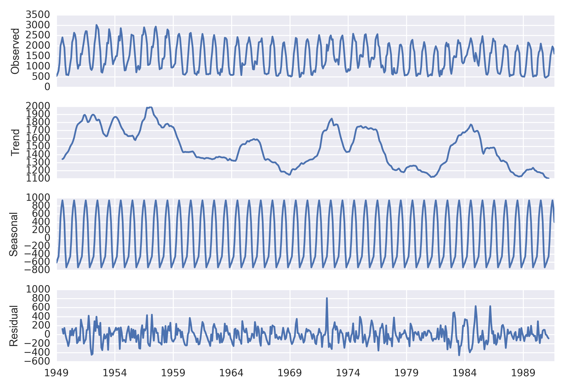  

decompose

Each component can then be accessed with:

residual = res.residual
seasonal = res.seasonal
trend = res.trend
print trend['1950':'1951']

1950-01-31    1441.591667  
1950-02-28    1468.133333  
1950-03-31    1499.883333  
1950-04-30    1521.466667  
1950-05-31    1540.633333  
1950-06-30    1572.079167  
1950-07-31    1611.412500  
1950-08-31    1666.541667  
1950-09-30    1720.658333  
1950-10-31    1759.700000  
1950-11-30    1780.408333  
1950-12-31    1789.491667  
1951-01-31    1800.950000  
1951-02-28    1810.950000  
1951-03-31    1819.616667  
1951-04-30    1848.866667  
1951-05-31    1889.850000  
1951-06-30    1895.979167  
1951-07-31    1878.858333  
1951-08-31    1841.137500  
1951-09-30    1806.308333  
1951-10-31    1807.850000  
1951-11-30    1826.516667  
1951-12-31    1856.683333  
Freq: M, Name: mean_va, dtype: float64  

If we want to determine if there is a simple monotonic trend in this data we can utilize the Mann-Kendall test for trend. This doesn’t appear to be available in scipy.stats or statsmodels yet. I came across a function written by Sat Kumar Tomer, the homepage with the software package seems to be gone, so I verified the output to implementations in R and uploaded to GitHub so it won’t disappear.

import numpy as np  
from scipy.stats import norm, mstats


def mk_test(x, alpha = 0.05):  
    """   
    Input:
        x:   a vector of data
        alpha: significance level (0.05 default)

    Output:
        trend: tells the trend (increasing, decreasing or no trend)
        h: True (if trend is present) or False (if trend is absence)
        p: p value of the significance test
        z: normalized test statistics 

    Examples
    --------
      >>> x = np.random.rand(100)
      >>> trend,h,p,z = mk_test(x,0.05) 
    """
    n = len(x)

    # calculate S 
    s = 0
    for k in range(n-1):
        for j in range(k+1,n):
            s += np.sign(x[j] - x[k])

    # calculate the unique data
    unique_x = np.unique(x)
    g = len(unique_x)

    # calculate the var(s)
    if n == g: # there is no tie
        var_s = (n*(n-1)*(2*n+5))/18
    else: # there are some ties in data
        tp = np.zeros(unique_x.shape)
        for i in range(len(unique_x)):
            tp[i] = sum(unique_x[i] == x)
        var_s = (n*(n-1)*(2*n+5) + np.sum(tp*(tp-1)*(2*tp+5)))/18

    if s>0:
        z = (s - 1)/np.sqrt(var_s)
    elif s == 0:
            z = 0
    elif s<0:
        z = (s + 1)/np.sqrt(var_s)

    # calculate the p_value
    p = 2*(1-norm.cdf(abs(z))) # two tail test
    h = abs(z) > norm.ppf(1-alpha/2) 

    if (z<0) and h:
        trend = 'decreasing'
    elif (z>0) and h:
        trend = 'increasing'
    else:
        trend = 'no trend'

    return trend, h, p, z

Let’s see if there is a trend direction in the first decade of data 1950-1960:

trend = res.trend['1950':'1960']  
test_trend,h,p,z = mk_test(trend,alpha=0.05)  
print test_trend, h  
print z, p  

decreasing True  
-4.05429896945 5.02848722452e-05

The test indicates a monotonic decreasing trend over the time period, with a Mann-Kendall Z stat = -4.05 and p<0.05.